Lei Feng Network Press: This article from the end compiler.
George Hotz and Comma.ai background:
George Hotz first cracked the iPhone in 2007 and became the first person to crack the Sony PS3 in 2010. After working internships at Google and Facebook, she stayed at Space for four months. In 2015, she joined the artificial intelligence startup Vicarious. In July of the same year, she left and founded Comma.ai in September. She studied autonomous driving technology in the garage and announced the challenge. Google, Mobileye, in April this year the company received 3.1 million US dollars of investment. On August 6th, George Hotz open sourced its research results such as source code and papers. (Thesis and source code can be clicked to download)
Original author Eder Santana, George Hotz. The following is the compilation of the full text:
The application of artificial intelligence in automatic driving, Comma.ai's strategy is to establish an agent to simulate the prediction of future road events to train the car to imitate human driving behavior and driving planning capabilities. This paper describes a method that we currently use for driving simulation to study Variational Autoencoders (VAEs) and generative adversarial networks (GANs) for roads. Video prediction cost function. Later, we trained a transition model based on this recurrent neural network (RNN).
The optimized model does not have a cost function in the pixel space, but the method we demonstrate can still achieve the prediction of multi-frame realistic pictures.
| IntroductionAuto-driving cars [1] is one of the most promising fields in the artificial intelligence research in the short-term. At this stage, the technology uses a lot of data with tags and rich context information that appear in the driving process. Given its perception and control complexities, once automated driving technology is realized, it will also develop many interesting technical topics, such as motion recognition and driving planning in video. At this stage, taking the camera as the main sensor, combined with visual processing and artificial intelligence technology to achieve automatic driving in the cost advantage.
Due to the development of deep learning and recursive neural networks, the interaction between virtual and reality is becoming more convenient. Vision-based control and reinforcement learning have been successful in the following literature [7][8][9][10] . This form of interaction allows us to repeatedly test the same scenario with different strategies and simulate all possible events to train neural network based controllers. For example, Alpha Go [9] uses deep convolutional neural network (CNN) to predict the probability of winning next time by constantly accumulating experience in playing games with himself. Go's game engine can simulate all possible evolutionary outcomes in the game and be used as a Markov Chain Tree search. Currently, if Go learns to play Torc[7] or Atari[8] with a game screen, it takes hours of training and learning.
Because the learning agent is difficult to achieve an exhaustive interaction with reality, there are currently two solutions. One is to manually develop a set of simulators, and the other is to train the ability to predict future scenarios . The former solution involves the definition of the rules of the physical world and the professional field of modeling the randomness of reality. However, such professional knowledge already covers all the information related to control and basically covers existing ones such as flight simulators [11]. Robot walking [12] and other fields.
We focus on the simulation of real-world scenarios by setting up human agents. A front camera is installed on the front windshield as input for the video stream.
In the early years, the training of the controller was simulated based on the state space of the physical agent [13]. Other models relying only on visual processing can only adapt to simple videos with low dimensional or texture features, such as games Atari [14] [16]. For videos with complex texture features, the motion is identified by passive video prediction [17].
This dissertation supplements existing literature related to video prediction. We let the controller itself train the model and predict realistic video scenes, calculate low-dimensional compression representations and convert them into corresponding actions. In the next section, we describe the datasets used to predict the video captured in real-time traffic conditions.
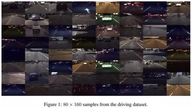
| DatasetsWe have open-sourced some of the autopilot test data used in this paper. The test data in the data set is consistent with comma.ai's self-driving car test platform using a consistent camera and sensor. We installed a Point Grey camera on the front windshield of Acura ILX 2016 and captured the road at 20hz. The released data set contains a total of 7.25 hours of driving data, which is divided into 11 videos. The video frame captures 160,320 pixels from the middle of the captured video. In addition to the video, the dataset also includes data from several sensors, which are measured at different frequencies, interpolating 100Hz. Example data includes vehicle speed, steering angle, GPS, gyroscope, and IMU. Specific details of data sets and measurement equipment can be obtained by visiting the synchronization site.
We record the timestamp when the sensor measures and captures the video frame, and use the test time and linear interpolation to synchronize the sensor and video data. We also released video and sensor raw data stored in HDF5 format, which was chosen because it is easier to use in machine learning and control software.
In this article, emphasis will be placed on video frames, steering angles, and car speeds. We obtained the 80160 image by downsampling the original data and performed a 1- to 1 pixel renormalizing of the image. This completes the preprocessing. The sample image is shown in Figure 1. In the next section we define the problems that this article aims to study.
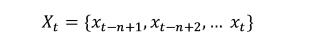
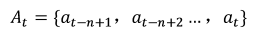
| Problem definitionXt represents the t-th frame of the data set, and Xt is the video representation of the frame length n:
St is the control signal and is directly related to the image frame:
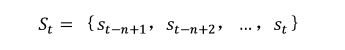
At corresponds to the vehicle speed and the steering angle.
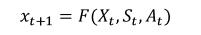
Define the evaluation function F when predicting the road image:
The prediction result of the next frame is:
Note that this definition is high-dimensional and the dimensions are interrelated, and similar problems in machine learning can occur, such as slow convergence or underfit [26].
Studies have shown [20] that when using a convolutional dynamic network, without proper regularization, the model performs well on a single set of data but has low prediction accuracy on the overall data. .
In the former method, the evaluation function F was directly trained by a simple, artificial video [14]. Recently, the paper [20] [17] shows that it is possible to predict the generation of video with high texture complexity, but it does not solve the transfer of motion conditions. The problem also does not generate a compact intermediate representation of the data. In other words, their models are not reduced in pixel sampling and do not have low-dimensional hidden coding, but are completely implemented through convolutional transformations. However, due to the high-dimensional dense space[18], the definitions of the probability, the filter, and the control output are ill-defined, and the compact intermediate representation studies us. The work is very important.
To the best of our knowledge, this is the first paper that attempts to predict subsequent frames of video from real-world highway scenarios. In this paper, we decided to segment the learning function F so that it can be debugged in blocks.
First, we learned that an Autoencoder embeds frame data xt into a Gaussian latent space (Zt).

Dimension 2048 is determined by experimental requirements. Variational Bayes [1] self-encoding (variational Autoencoding Bayes) enforces Gaussian assumptions. The first step is to simplify the learning transfer in pixel space to learning in the latent space. In addition, suppose that the autoencoder can correctly learn the Gaussianity of the hidden layer, so long as the transfer model can guarantee not to leave. By embedding high-density areas of space, we can simulate realistic video images. The hypersphere radius of the high-density region is Ï, which is a function of the embedding spatial dimension and Gaussian prior variance. In the next section we will begin to introduce the Autoencoder and transfer model in detail.
| Driving simulatorConsidering the complexity of the problem, we do not consider the End-to-End method, but use a separate network to learn video prediction. The proposed architecture is based on two models: one is the use of Autoencoder for dimensionality reduction and the other is the use of an RNN for transition learning. The complete model is shown in Figure 2.
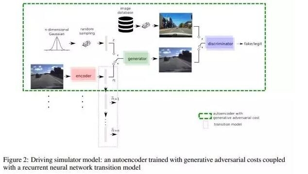
Autoencoder We choose a model with hidden layer as Gaussian probability distribution to learn data embedding, especially to avoid the low-probability discontinuity area where the hypersphere is concentrated in the origin. This area will hinder the hidden layer Continuous transformation model learning. Variational Autoencoder[1] and related work [19][21] used the Gaussian prior model to complete the learning of the generative model in the hidden layer of the original data. However, Gaussian assumptions in the original data space are applicable to the processing of natural images, and thus the VAE prediction results may look vague (see Figure 3). On the other hand, generating the countermeasure network (GAN) [22] and related work [2] [3] will learn the cost function of the generated model together with the generator. Therefore, alternate training of generative and discriminator networks is possible.
The generative generation model converts sample data distributed in the hidden layer to the data set, discriminator discrimination network discerns samples in the data set from all samples of the generator, but the generator can act as a fool discriminator, so the discriminator can also be regarded as It is a cost function of the generator.
We not only need to learn the generator from the hidden layer to the road image space, but also can feedback the road image coding back to the hidden layer, so we need to combine the VAE with the GAN network. Intuitively, a simple way is to combine the VAE method directly with a cost function. In Donahue et.al's paper [23], a two-way GAN network with a learning generation model and bijective transform coding is proposed. Lamb et al. [24] proposed discriminative generative networks and used the previously trained classifier feature differences as part of the cost function. Finally, Larsen et.al [25] proposed to train the VAE and GAN networks together so that the encoder can simultaneously optimize the Gaussian prior model of the hidden layer and the similarity extracted from the GAN network. The generator takes a random sample output from the hidden layer as an input and outputs an encoder network. After optimization, it can fool the discriminator and minimize the similarity between the original image and the decoded image. The discriminator is always trained to distinguish the authenticity of the input picture - authenticity.
We use the method of Larsen et.al.[25] to train the Autoencoder. The schematic in Figure 2 shows this model. In the paper [25], encoder (Enc), generator (Gen) and discriminator (Dis) networks optimized in the paper, the following cost function values ​​are minimized:

In the above formula,
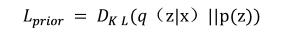
The Kullback-Liebler divergence that satisfies both the encoded output distribution q(z|x) and the prior distribution p(z) is a VAE regularization matrix, and p(z) satisfies the N(0,1) Gaussian distribution. We use reparemetrization to optimize Its regularizer, therefore, always satisfies z = μ + ∈σ during the training process, and satisfies z = μ during the test (where μ and σ are the output of the coded network, and ∈ is the same Gaussian random as μ and σ). vector)
The second term is a calculated error value, which represents the hidden activation value of the layer 1 in the discrimination network. The value is computed using the legal image x and the corresponding coded-re-decoded value Gen(Dis(x)) .
Assumptions:
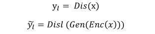
You can get:
In the training process, Dis is usually handled in a constant way to avoid steps that are too cumbersome.
Finally, LGAN is the cost of generating a confrontation network (GAN) [22]. The cost function represents the game relationship between Gen and Dis. When training Dis, Enc and Gen always maintain a fixed value:

u is a random variable that satisfies the normal distribution N(0,1). The first part of the formula is the log likelihood function of Dis, which is used to determine the legal image. The remaining two parts are the random vector u or the code value z. = The logarithm of Enc(x), used to determine if it is a fake image sample.
When training Gen, Dis and Enc always have a fixed value:

This indicates that Gen can determine the network by fool Dis. [25] The second item in the equation, Enc(x), is usually set to 0 during training.
We have trained the Autoencoder 200 times, each iteration contains 10,000 gradient updates, and the size of the increment is 64. As described in the previous section, the samples are randomly sampled from the driving data. We use Adam for optimization [4], self-encoder network architecture reference Radford et.al [3]. The generator consists of four layers of unrolled base layers, followed by normalization of samples followed by activation of leaky-ReLU . Discriminators and encoders consist of a multilayer volume base layer, and the first layer is followed by normalization of the sample. The activation function used here is ReLU. Disl is the network output of the decoder's third layer of the base layer, and then the sample normalization and ReLU operations. The discriminator's output size is 1, its cost function is a binary cross-entropy function, and the output size of the coded network is 2048. Such a compact representation compresses to 1/16 of the original data dimension. Detailed information can be viewed in Figure 2 or this paper's synchronization code. Sample encoding-re-decoding and target images are shown in Figure 3.
After training the Autoencoder, we fixed all the weights and used Enc as a preprocessing step for the training transformation model. We will discuss the transformation model in the next section.
Transition model
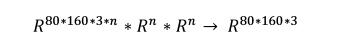
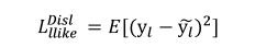
After training the Autoencoder, we got the data set for the transformation. We use Enc to train the RNN: zt, ht, ct -> Zt+1 for xt -> zt to represent the transformation of the coding space.
W, V, U, A in the formula are training weights, ht is the hidden state of the RNN, ct directly controls the vehicle speed and steering angle signals, and LSTM, GRU, and multiplication iterations between ct and zt are For further research in the future, the cost function now used to optimize the training weights is the mean square error (MSE):
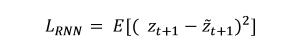
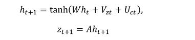
Obviously this formula is optimal because we have imposed the Lprior's Gaussian constraint on the distribution of the encoding z when training the Autoencoder. In other words, the mean square error will equal the logarithm of a normally distributed random variable. If the predicted coding value is:

The estimated frame of the picture can be expressed as
We use a video sequence with a frame length of 15 to train the transformation model. After the first 5 frames of learning results are output, it will be used as the input of the last 10 frames of learning network. That is, after we use the Enc(xt) function to calculate z1,...,z5, continue. As a follow-up input, get

Feedback continues as input. In the RNN literature, it is known as RNN hallucination that the output is fed back as input. In order to avoid complex operations, we continue to use the former output feedback as the gradient in the input process is set to zero.
| Test resultsIn this study, we spent most of our energy on how to make the Autoencoding architecture retain the texture features of the road. As mentioned above, we studied different cost functions. Although they all have similar error, the GAN network is used. The cost function still got the best visual result. As shown in Figure 3, we show two decoded pictures generated by two training models corresponding to different cost functions. As expected, the images generated by the MSE-based neural network are blurred, making multiple lane identification lines erroneous. The identification became a long single lane.
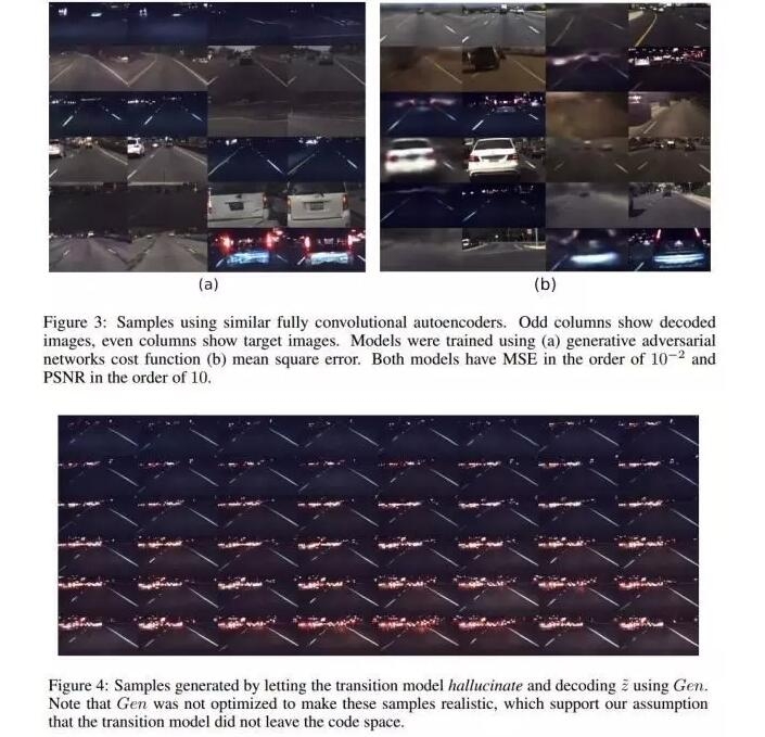
In addition, the fuzzy reconstruction can not preserve the edge of the image of the preceding vehicle. Therefore, the main reason why this method cannot be used for promotion is that it is difficult to achieve distance measurement and estimation of the distance to the preceding vehicle. On the other hand, using MSE to learn to draw curved line speeds is faster than a network-based model. It may be possible to avoid this problem when learning to encode pixels with car steering angle information. We will keep this question for future study.
Once we have a good Autoencoder, we can start training the transformation model. The predicted picture frame results are shown in Fig. 4. We used the 5Hz video conversion model for training. After learning, the conversion model can always maintain the road picture structure after 100 frames. When sampling from the conversion model with different seed frames, we observed driving events that included passing the lane line, approaching the preceding vehicle, and driving ahead. However, the model could not simulate the curve scenario. When we initialize the conversion model with image frames running on a curve, the conversion model quickly straightens the lane lines and restarts the analog straight-line driving. In this model, we can still learn the conversion of video, even though there is no accurate optimization cost function in the pixel space. We also believe that relying on more powerful conversion models (such as deep RNN, LSTM, GRU) and contextual encoding (sensor-assisted video sampling plus steering angle and speed) will lead to more realistic simulations.
The data set released in this paper contains all necessary sensors for this method during the experiment.
| ConclusionThis paper introduces the preliminary research results of comma.ai in learning the automobile driving simulator, based on the video prediction model of Autoencoder and RNN. We do not associate End-to-End learning with all things. Instead, we first train the Autoencoder using a cost function based on the Genesis GAN (GAN) to generate realistic road images. Then we A RNN transformation model was trained in the embedding space. Although the results of the Autoencoder as well as the conversion model appear to be very realistic, more research is needed to simulate all the events related to the driving process. In order to stimulate deeper research on automated driving, we have released this driving dataset that includes video sampling and sensor data such as car speed and steering angle, and has open sourced the neural network source code that is currently being trained.
references
[1] Diederik P Kingma and Max Welling, “Auto-encoding variational bayes,†arXiv preprint
arXiv: 1312.6114, 2013.
[2] Emily L Denton, Soumith Chintala, Rob Fergus, et al., “Deep generative image models using laplacian pyramid of adversarial networks,†in Advances in Neural Information Processing Systems, 2015.
[3] Radford, Alec, Luke Metz, and Soumith Chintala. "Unsupervised representation learning with deep convolutional generative adversarial networks." arXiv preprint arXiv: 1510.13614, 2015.
[4] Diederik Kingma and Jimmy Ba, “Adam: A method for stochastic optimization.†arXiv
Preprint arXiv: 1412.6980, 2014.
[5] Ian Goodfellow, Jean Pouget-Abadie, Mehdi Mirza, Bing Xu, David Warde-Farley, Sherjil Ozair, Aaron Courville, and Yoshua Bengio, “Generative adversarial nets,†in Advances in Neural Information Processing Systems, 2014.
[6] Alireza Makhzani, Jonathon Shlens, Navdeep Jaitly, and Ian Goodfellow, “Adversarial Autoencoders,†arXiv preprint arXiv: 1511.05644, 2015.
[7] Jan Koutn Ì Ä±k, Giuseppe Cuccu, Jurgen Schmidhuber, and Faustino Gomez, “Evolving large-scale neural networks for vision-based reinforcement learning,†Proceedings of the 15th annual conference on Genetic and Evolutionary computation, 2013.
[8] Volodymyr Mnih, Koray Kavukcuoglu, David Silver, et al., “Human-level control through deep reinforcement learning,†Nature, 2015.
[9] David Silver, Aja Huang, Chris Maddison, et al., “Mastering the game of Go with deep neural networks and tree search,†Nature, 2016.
[10] Sergey Levine, Peter Pastor, Alex Krizhevsky, and Deirdre Quillen, “Learning Hand-Eye Coordination for Robotic Grasping with Deep Learning and Large-Scale Data Collection,â€
arXiv preprint arXiv: 1603.02199, 2016.
[11] Brian L Stevens, Frank L Lewis and Eric N Johnson, “Aircraft Control and Simulation: Dynamics, Controls Design, and Autonomous Systems,†John Wiley & Sons, 2015.
[12] Eric R Westervelt, Jessy W Grizzle, Christine Chevallereau, et al., “Feedback control of dynamic bipedal robot locomotion,†CRC press, 2007.
[13] HJ Kim, Michael I Jordan, Shankar Sastry, Andrew Y Ng, “Autonomous helicopter flight via reinforcement learning,†Advances in neural information processing systems, 2003.
[14] Junhyuk Oh, Xiaoxiao Guo, Honglak Lee, et al., “Action-conditional video prediction using deep networks in atari games,†Advances in Neural Information Processing Systems, 2015.
[15] Manuel Watter, Jost Springenberg, Joschka Boedecker and Martin Riedmiller, “Embed to control: A locally linear latent dynamics model for control from raw images,†Advances in Neural Information Processing Systems, 2015.
[16] Jurgen Schmidhuber, “On learning to think: Algorithmic information theory for novel com- binations of reinforcement learning controllers and recurrent neural world models,†arXiv preprint arXiv: 1511.09249, 2015.
[17] Michael Mathieu, Camille Couprie and Yann LeCun, “Deep multi-scale video prediction beyond mean square error,†arXiv preprint arXiv: 1510.154440, 2015.7
[18] Ramon van Handel, "Probability in high dimension," DTIC Document, 2014.
[19] Eder Santana, Matthew Emigh and Jose C Principe, “Information Theoretic-Learning Autoencoder,†arXiv preprint arXiv:1603.06653, 2016.
[20] Eder Santana, Matthew Emigh and Jose C Principe, “Exploiting Spatio-Temporal Dynamics for Deep Predictive Coding,†Under Review, 2016.
[21] Alireza Makhzani, Jonathon Shlens, Navdeep Jaitly and Ian Goodfellow, “Adversarial Autoencodersâ€, arXiv preprint arXiv: 1511.05644, 2015.
[22] Ian Goodfellow, Jean Pouget-Abadie, Mehdi Mirza, et al., “Generative adversarial nets,†Advances in Neural Information Processing Systems, 2014.
[23] Jeff Donahue, Philipp Krahenb ̈ uhl and Trevor Darrell, “Adversarial Feature Learning,†̈ arXiv preprint arXiv: 1605.09782, 2016.
[24] Alex Lamb, Vincent Dumoulin Vincent and Aaron Courville, "Discriminative Regularization for Generative Models," arXiv preprint arXiv: 1602.03220, 2016.
[25] Anders Boesen Lindbo Larsen, Søren Kaae Sønderby, Hugo Larochelle and Ole Winther, “Autoencoding beyond pixels using a learned similarity metric,†arXiv preprint arXiv: 1512.09300, 2015.
[26] Jose C Principe, Neil R Euliano, W Cur Lefebvre, “Neural and adaptive systems: fundamentals through simulations with CD-ROM†John Wiley
Lei Feng Network (search "Lei Feng Network" public concern) Note: Reprinted, please contact the authorization, and retain the source and author, not to delete the content.